 ecbyts
Walk the corporate GHG inventory from collection to reporting
About 6 min read
- Guide
- Audio
- Tour
Eleven steps take a corporate greenhouse gas (GHG) inventory from who answers for each unit to the workbook and the MAC curve. Sample spreadsheets with fictitious data.
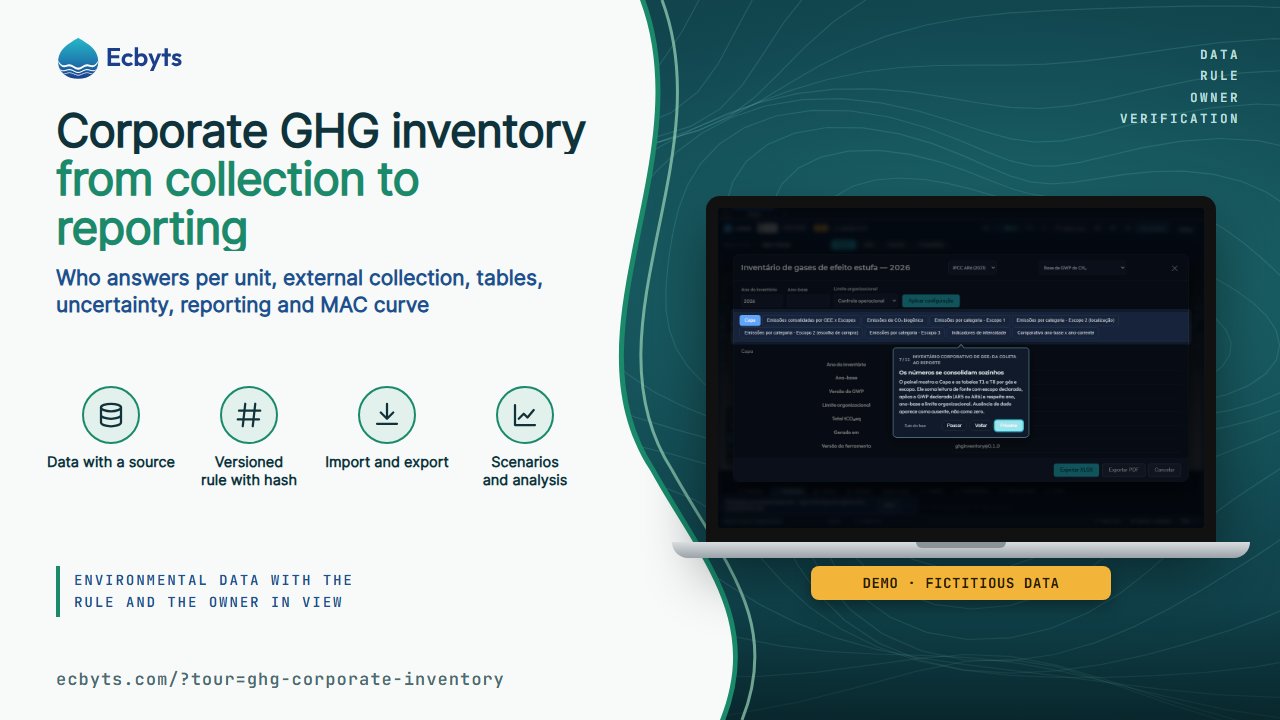
A company greenhouse gas (GHG) inventory only stands when every number has an owner, a source and a period, and that calculation often stays locked in spreadsheets nobody can rebuild later. The Corporate GHG inventory: from collection to reporting tour walks the whole cycle in 11 steps in ecbyts: who answers for each unit, the reading made by someone outside the app, consolidation into a single model, the tables, the reporting workbook, the report, the MAC curve and uncertainty. The walkthrough opens the real screens of the app and does not simulate data.
What the tour shows, step by step
- The whole path. The walkthrough starts at the app header and presents the corporate inventory cycle. Each following step opens a real screen of the app.
- Who answers for each unit. In the Collection inbox panel, each planned reading becomes a link: the campaign carries the unit and the period, and the link carries the element and the parameter. Generate one link per reading and send it to whoever takes the measurement. The respondent does not create an account. People who already have an account can be invited as responsible for the project or the campaign, and the link only counts after the person accepts.
- What the outside person fills in. The link opens a page with no sign-up: date, whether the substance was detected, reading, unit, method, laboratory, detection limit and notes. The person receives a protocol number. The data waits in a holding area on the server and does not enter the model until you accept it. There is no automatic check of what was sent.
- Batch collection through the kit spreadsheets. Inside Import Data, the collection kit offers nine spreadsheets with fictitious data, one per subject. The GHG ones are electricity, stationary fuels, fleet and refrigerant gases. Download the ones you need, fill them in with the units and send them back. There is no button to download them all at once.
- The spreadsheet becomes data with a source. When you import, the wizard reads the columns, shows what it recognized and points out errors line by line. Nothing is saved before you confirm. Each accepted line keeps its source: unit, date, parameter and unit of measure. Changing the unit of measure is not formatting: it changes the number.
- One private model per company. Back in Collection inbox, each accepted reading becomes an observation in the model with the protocol number and the record of who approved it. The company inventory is one model. A model saved in the cloud belongs to the organization and has restricted access. The external link receives only the reading, never the model.
- The numbers add up on their own. The panel shows the cover and tables T1 to T8 by gas and scope. It adds the source reading with the declared scope, applies the chosen global warming potential (GWP), between AR5 and AR6, and respects the year, the baseline year and the organizational boundary. A missing reading appears as missing, not as zero.
- Export in the program format. Export XLSX generates the workbook with nine sheets: cover and T1 to T8, in the inventory program format. That file is the one that goes to the review. Export PDF only warns that the document is not produced in this version. And the way back is not automatic, because the app does not import this spreadsheet back.
- The inventory report. The report is the very cover plus the tables: owner, period, baseline year, organizational boundary, GWP basis and each gas by scope. It summarizes the data version. It is not independent verification nor a public registry, and whoever signs the verification stays outside the app.
- From the inventory to the MAC curve projects. The MAC curve ranks measures by efficiency, meaning cost per tonne abated, from CAPEX, OPEX and reduction per period. Click the information button (ⓘ) next to a field to open the field metadata panel, with the meaning and the source of the data. It is the only step that only moves on when that panel opens. Inventory values do not enter the curve on their own: you reference them when you register a measure.
- How much uncertainty the number carries. The uncertainty screen applies the IPCC 2006 method, Volume 1, Chapter 3: combined uncertainty by category and gas, Monte Carlo simulation and reporting in the Table 3.3 form. There is an official example to practice with, Finland 2003, without touching your data.
Fictitious data. The tour does not make up numbers: it opens the screens of the model that is already open. What is fictitious are the collection kit spreadsheets, which carry a few sample rows to show the format of each column. In a real inventory you fill the same spreadsheets with the units, the measurements and the lab reports of the operation, and the source of every reading stays recorded in the model.
What this tour is not
- It is not a batch collection campaign. External collection is one link per planned reading, generated and accepted one at a time. There is no mass invitation, no respondent registered per unit and no portal with a task list for the whole company. Generating a link, accepting a reading and inviting a responsible person require a signed-in session and a model saved in the organization.
- It does not generate an inventory PDF. The PDF button only warns that the document is not produced in this version; the deliverable is the nine-sheet XLSX.
- It does not import the T1 to T8 spreadsheet back. The file is an output, not an input: the app does not reread the exported spreadsheet to recheck or reprocess the numbers.
- It does not perform the independent verification. No screen of the app issues a verification statement or a third-party opinion; the external review happens outside and is not automated.
- It does not link the MAC curve to the inventory on its own. You reference the measure when you register it; there is no automatic read of the consolidated emissions.
- It does not group the panel by organizational unit. Tables T1 to T8 add up by gas and scope, with the category inside each scope. The unit appears when you register the source and in the collection, but it does not become a grouping in the panel.
- Uncertainty is a separate calculator. You type the rows and the IPCC method returns the result; the panel does not pull the inventory readings by itself.
How to practice
Open the tour and move on with Next. There are 11 steps, about 12 minutes, and the walkthrough saves nothing to the model. All you need is an open model, even an empty one, because the screens open with the data that already exists. The tour requires no paid plan. To really generate a collection link, accept a reading or invite a responsible person, sign in to your account and save the model in the organization.